In order to visualize the data with traditional tools such as QGIS we add to table Trip a column Trajectory of type geometry containing the trajectory of the trips.

ALTER TABLE Trips ADD COLUMN Trajectory geometry;
UPDATE Trips
SET Trajectory = trajectory(Trip);

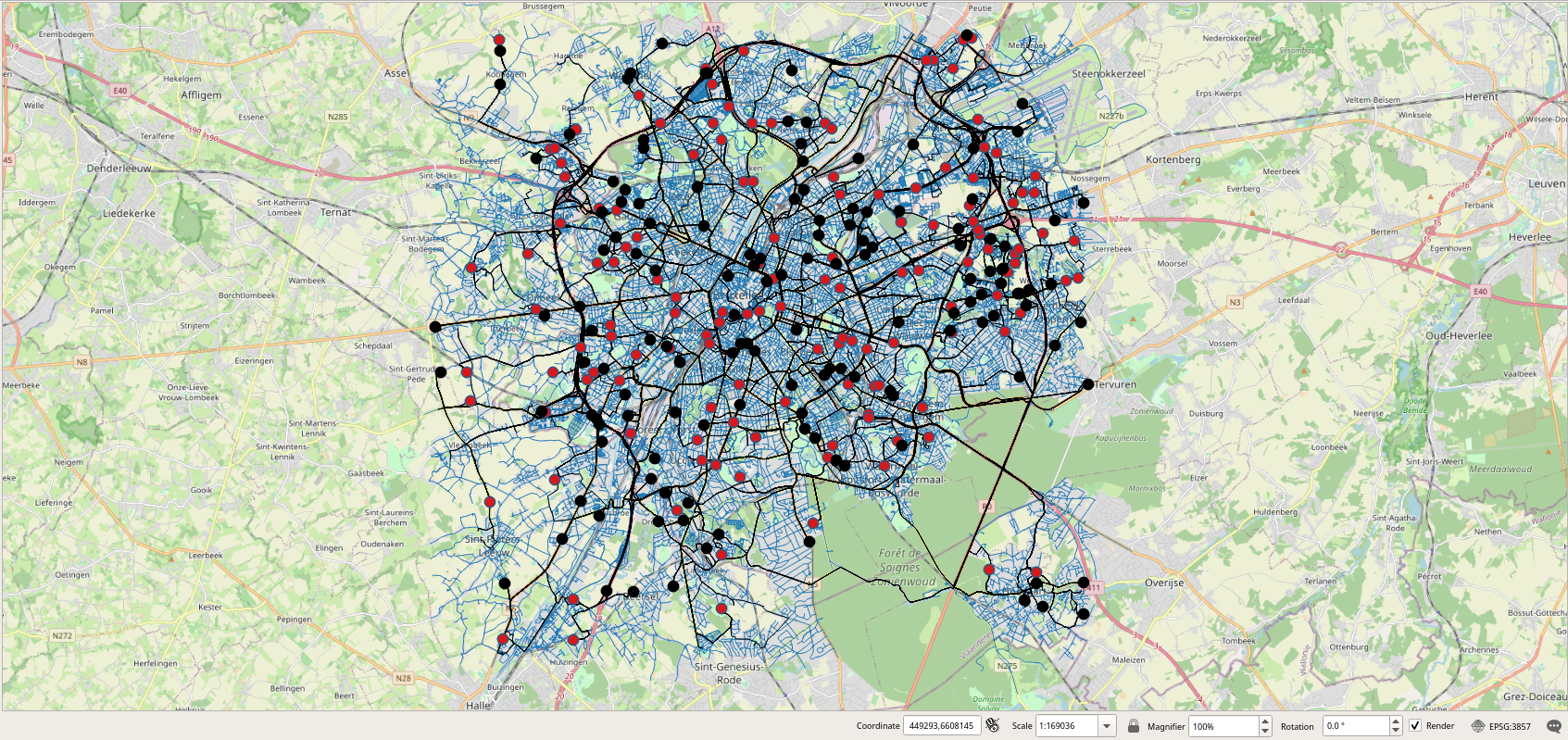
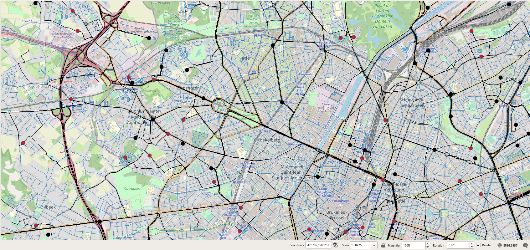
The visualization of the trajectories in QGIS is given in Figure 1.2, “Visualization of the trips in QGIS. The streets are shown in blue, the trips are shown in black, the home nodes in black and the work nodes in red.”. As we will explain in Chapter 2, Generating Realistic Trajectory Datasets this synthetic dataset models people using their car for going from home to work in the morning, from work to home in the afternoon, as well as doing some additional leisure trips at evenings or weekends.

Figure 1.2. Visualization of the trips in QGIS. The streets are shown in blue, the trips are shown in black, the home nodes in black and the work nodes in red.

In order to know the total number of trips as well as the number of trips we can issue the following queries.

SELECT count(*) FROM Trips;
-- 1672
SELECT count(*) FROM Trips WHERE GeometryType(Trajectory) = 'POINT';
-- 0
SELECT count(*) FROM Trips WHERE GeometryType(Trajectory) = 'LINESTRING';
-- 1672

We can also determine the spatiotemporal extent of the data using the following query.

SELECT extent(Trip) from Trips;
/* SRID=3857;STBOX XT(((469715.0960907607,6577078.768286072),
    (500997.56505993055,6607214.0038881665)),
    [2020-06-01 08:01:16.984+02, 2020-06-05 01:40:04.281127+02]) */

We continue investigating the data set by computing the maximum number of concurrent trips over the whole period

SELECT maxValue(tcount(Trip)) FROM Trips;
-- 51

the average sampling rate

SELECT AVG(duration(Trip)/numInstants(Trip)) FROM Trips;
-- 00:00:01.370537

and the total travelled distance in kilometers of all trips:

SELECT SUM(length(Trip)) / 1e3 as TotalLengthKm FROM Trips;
-- 24209.259034796323

Now we want to know the average duration of a trip.

SELECT AVG(duration(Trip)) FROM Trips;
-- 00:25:09.065361

This following query tells us the length in kilometers and the duration of each trip.

SELECT tripId, length(Trip) / 1e3 AS lengthKm, duration(Trip) AS duration
FROM Trips ORDER BY duration;

The following query produces a histogram of trip length.

WITH Bins(BinNo, BinRange) AS (
  SELECT 1, floatspan '[0, 1)' UNION
  SELECT 2, floatspan '[1, 2)' UNION
  SELECT 3, floatspan '[2, 5)' UNION
  SELECT 4, floatspan '[5, 10)' UNION
  SELECT 5, floatspan '[10, 50)' UNION
  SELECT 6, floatspan '[50, 100)' ),
Histogram AS (
  SELECT BinNo, BinRange, COUNT(TripId) AS Freq
  FROM Bins LEFT OUTER JOIN Trips ON length(trip) / 1e3 <@ BinRange
  GROUP BY BinNo, BinRange
  ORDER BY BinNo, BinRange )
SELECT BinNo, BinRange, Freq,
  repeat('■', ( Freq::float / MAX(Freq) OVER () * 30 )::int ) AS bar
FROM Histogram;

The result of the above query is given next.

 BinNo | BinRange  | Freq |              bar
-------+-----------+------+--------------------------------
     1 | [0, 1)    |   41 | ■
     2 | [1, 2)    |   91 | ■■■
     3 | [2, 5)    |  329 | ■■■■■■■■■■■
     4 | [5, 10)   |  294 | ■■■■■■■■■■
     5 | [10, 50)  |  909 | ■■■■■■■■■■■■■■■■■■■■■■■■■■■■■■
     6 | [50, 100) |    8 |