As we did at the beginning of this chapter, we load the OSM data from Brussels into PostgreSQL with the following command.

osm2pgsql --create --database brussels --host localhost brussels.osm

The table planet_osm_line contains all linear features imported from OSM, in particular road data, but also many other features which are not relevant for our use case such as pedestrian paths, cycling ways, train ways, electric lines, etc. Therefore, we use the attribute highway to extract the roads from this table. We first create a table containing the road types we are interested in and associate to them a priority, a maximum speed, and a category as follows.

DROP TABLE IF EXISTS RoadTypes;
CREATE TABLE RoadTypes(id int PRIMARY KEY, type text, priority float, maxspeed float,
category int);
INSERT INTO RoadTypes VALUES
(101, 'motorway', 1.0, 120, 1),
(102, 'motorway_link', 1.0, 120, 1),
(103, 'motorway_junction', 1.0, 120, 1),
(104, 'trunk', 1.05, 120, 1),
(105, 'trunk_link', 1.05, 120, 1),
(106, 'primary', 1.15, 90, 2),
(107, 'primary_link', 1.15, 90, 1),
(108, 'secondary', 1.5, 70, 2),
(109, 'secondary_link', 1.5, 70, 2),
(110, 'tertiary', 1.75, 50, 2),
(111, 'tertiary_link', 1.75, 50, 2),
(112, 'residential', 2.5, 30, 3),
(113, 'living_street', 3.0, 20, 3),
(114, 'unclassified', 3.0, 20, 3),
(115, 'service', 4.0, 20, 3),
(116, 'services', 4.0, 20, 3);

Then, we create a table that contains the roads corresponding to one of the above types as follows.

DROP TABLE IF EXISTS Roads;
CREATE TABLE Roads AS
SELECT osm_id, admin_level, bridge, cutting, highway, junction, name, oneway, operator,
ref, route, surface, toll, tracktype, tunnel, width, way AS Geom
FROM planet_osm_line
WHERE highway IN (SELECT type FROM RoadTypes);

CREATE INDEX Roads_geom_idx ON Roads USING GiST(Geom);

We then create a table that contains all intersections between two roads as follows:

DROP TABLE IF EXISTS Intersections;
CREATE TABLE Intersections AS
WITH Temp1 AS (
  SELECT ST_Intersection(a.Geom, b.Geom) AS Geom
  FROM Roads a, Roads b
  WHERE a.osm_id < b.osm_id AND ST_Intersects(a.Geom, b.Geom) ),
Temp2 AS (
  SELECT DISTINCT Geom
  FROM Temp1
  WHERE geometrytype(Geom) = 'POINT'
  UNION
  SELECT (ST_DumpPoints(Geom)).Geom
  FROM Temp1
  WHERE geometrytype(Geom) = 'MULTIPOINT' )
SELECT ROW_NUMBER() OVER () AS id, Geom
FROM Temp2;

CREATE INDEX Intersections_geom_idx ON Intersections USING GIST(Geom);

The temporary table Temp1 computes all intersections between two different roads, while the temporary table Temp2 selects all intersections of type point and splits the intersections of type multipoint into the component points with the function ST_DumpPoints. Finally, the last query adds a sequence identifier to the resulting intersections.

Our next task is to use the table Intersections we have just created to split the roads. This is done as follows.

DROP TABLE IF EXISTS Segments;
CREATE TABLE Segments AS
SELECT DISTINCT osm_id, (ST_Dump(ST_Split(R.Geom, I.Geom))).Geom
FROM Roads R, Intersections I
WHERE ST_Intersects(R.Geom, I.Geom);

CREATE INDEX Segments_geom_idx ON Segments USING GIST(Geom);

The function ST_Split breaks the geometry of a road using an intersection and the function ST_Dump obtains the individual segments resulting from the splitting. However, as shown in the following query, there are duplicate segments with distinct osm_id.

SELECT S1.osm_id, S2.osm_id
FROM Segments S1, Segments S2
WHERE S1.osm_id < S2.osm_id AND ST_Intersects(S1.Geom, S2.Geom) AND 
  ST_Equals(S1.Geom, S2.Geom);
-- 490493551  740404156
-- 490493551  740404157

We can remove those duplicates segments with the following query, which keeps arbitrarily the smaller osm_id.

DELETE FROM Segments S1
USING Segments S2
WHERE S1.osm_id > S2.osm_id AND ST_Equals(S1.Geom, S2.Geom);

We can obtain some characteristics of the segments with the following queries.

SELECT DISTINCT geometrytype(Geom) FROM Segments;
-- "LINESTRING"

SELECT MIN(ST_NPoints(Geom)), max(ST_NPoints(Geom)) FROM Segments;
-- 2	283

Now we are ready to obtain a first set of nodes for our graph.

DROP TABLE IF EXISTS TempNodes;
CREATE TABLE TempNodes AS
WITH Temp(Geom) AS (
  SELECT ST_StartPoint(Geom) FROM Segments UNION
  SELECT ST_EndPoint(Geom) FROM Segments )
SELECT ROW_NUMBER() OVER () AS id, Geom
FROM Temp;

CREATE INDEX TempNodes_geom_idx ON TempNodes USING GIST(Geom);

The above query select as nodes the start and the end points of the segments and assigns to each of them a sequence identifier. We construct next the set of edges of our graph as follows.

DROP TABLE IF EXISTS Edges;
CREATE TABLE Edges(id bigint, osm_id bigint, tag_id int, length_m float, source bigint,
  target bigint, cost_s float, reverse_cost_s float, one_way int, maxspeed float,
  priority float, Geom geometry);
INSERT INTO Edges(id, osm_id, source, target, Geom, length_m)
SELECT ROW_NUMBER() OVER () AS id, S.osm_id, n1.id AS source, n2.id AS target, S.Geom,
  ST_Length(S.Geom) AS length_m
FROM Segments S, TempNodes n1, TempNodes n2
WHERE ST_Intersects(ST_StartPoint(S.Geom), n1.Geom) AND
  ST_Intersects(ST_EndPoint(S.Geom), n2.Geom);

CREATE UNIQUE INDEX Edges_id_idx ON Edges USING BTREE(id);
CREATE INDEX Edges_geom_index ON Edges USING GiST(Geom);

The above query connects the segments obtained previously to the source and target nodes. We can verify that all edges were connected correctly to their source and target nodes using the following query.

SELECT count(*) FROM Edges WHERE source IS NULL OR target IS NULL;
-- 0

Now we can fill the other attributes of the edges. We start first with the attributes tag_id, priority, and maxspeed, which are obtained from the table RoadTypes using the attribute highway.

UPDATE Edges e
SET tag_id = t.id, priority = t.priority, maxspeed = t.maxSpeed
FROM Roads R, RoadTypes t
WHERE e.osm_id = R.osm_id AND R.highway = t.type;

We continue with the attribute one_way according to the semantics stated in the OSM documentation.

UPDATE Edges e
SET one_way = CASE
  WHEN R.oneway = 'yes' OR R.oneway = 'true' OR R.oneway = '1' THEN 1 -- Yes
  WHEN R.oneway = 'no' OR R.oneway = 'false' OR R.oneway = '0' THEN 2 -- No
  WHEN R.oneway = 'reversible' THEN 3 -- Reversible
  WHEN R.oneway = '-1' OR R.oneway = 'reversed' THEN -1 -- Reversed
  WHEN R.oneway IS NULL THEN 0 -- Unknown
  END
FROM Roads R
WHERE e.osm_id = R.osm_id;

We compute the implied one way restriction based on OSM documentation as follows.

UPDATE Edges e
SET one_way = 1
FROM Roads R
WHERE e.osm_id = R.osm_id AND R.oneway IS NULL AND
  (R.junction = 'roundabout' OR R.highway = 'motorway');

Finally, we compute the cost and reverse cost in seconds according to the length and the maximum speed of the edge.

UPDATE Edges e SET
cost_s = CASE
  WHEN one_way = -1 THEN - length_m / (maxspeed / 3.6)
  ELSE length_m / (maxspeed / 3.6)
  END,
reverse_cost_s = CASE
  WHEN one_way = 1 THEN - length_m / (maxspeed / 3.6)
  ELSE length_m / (maxspeed / 3.6)
  END;

Our last task is to compute the strongly connected components of the graph. This is necessary to ensure that there is a path between every couple of arbritrary nodes in the graph.

DROP TABLE IF EXISTS Nodes;
CREATE TABLE Nodes AS
WITH Components AS (
  SELECT * FROM pgr_strongComponents(
    'SELECT id, source, target, length_m AS cost, '
    'length_m * sign(reverse_cost_s) AS reverse_cost FROM Edges') ),
LargestComponent AS (
  SELECT component, count(*) FROM Components
  GROUP BY component ORDER BY count(*) DESC LIMIT 1 ),
Connected AS (
  SELECT Geom
  FROM TempNodes n, LargestComponent L, Components C
  WHERE n.id = C.node AND C.component = L.component )
SELECT ROW_NUMBER() OVER () AS id, Geom
FROM Connected;

CREATE UNIQUE INDEX Nodes_id_idx ON Nodes USING BTREE(id);
CREATE INDEX Nodes_geom_idx ON Nodes USING GiST(Geom);

The temporary table Components is obtained by calling the function pgr_strongComponents from pgRouting, the temporary table LargestComponent selects the largest component from the previous table, and the temporary table Connected selects all nodes that belong to the largest component. Finally, the last query assigns a sequence identifier to all nodes.

Now that we computed the nodes of the graph, we need to link the edges with the identifiers of these nodes. This is done as follows.

UPDATE Edges SET source = NULL, target = NULL;

UPDATE Edges e SET
  source = n1.id, target = n2.id
FROM Nodes n1, Nodes n2
WHERE ST_Intersects(e.Geom, n1.Geom) AND ST_StartPoint(e.Geom) = n1.Geom AND
  ST_Intersects(e.Geom, n2.Geom) AND ST_EndPoint(e.Geom) = n2.Geom;

We first set the identifiers of the source and target nodes to NULL before connecting them to the identifiers of the node. Finally, we delete the edges whose source or target node has been removed.

DELETE FROM Edges WHERE source IS NULL OR target IS NULL;
-- DELETE 1080

In order to compare the graph we have just obtained with the one obtained by osm2pgrouting we can issue the following queries.

SELECT count(*) FROM Ways;
-- 83017
SELECT count(*) FROM Edges;
-- 81073
SELECT count(*) FROM Ways_vertices_pgr;
-- 66832
SELECT count(*) FROM Nodes;
-- 45494

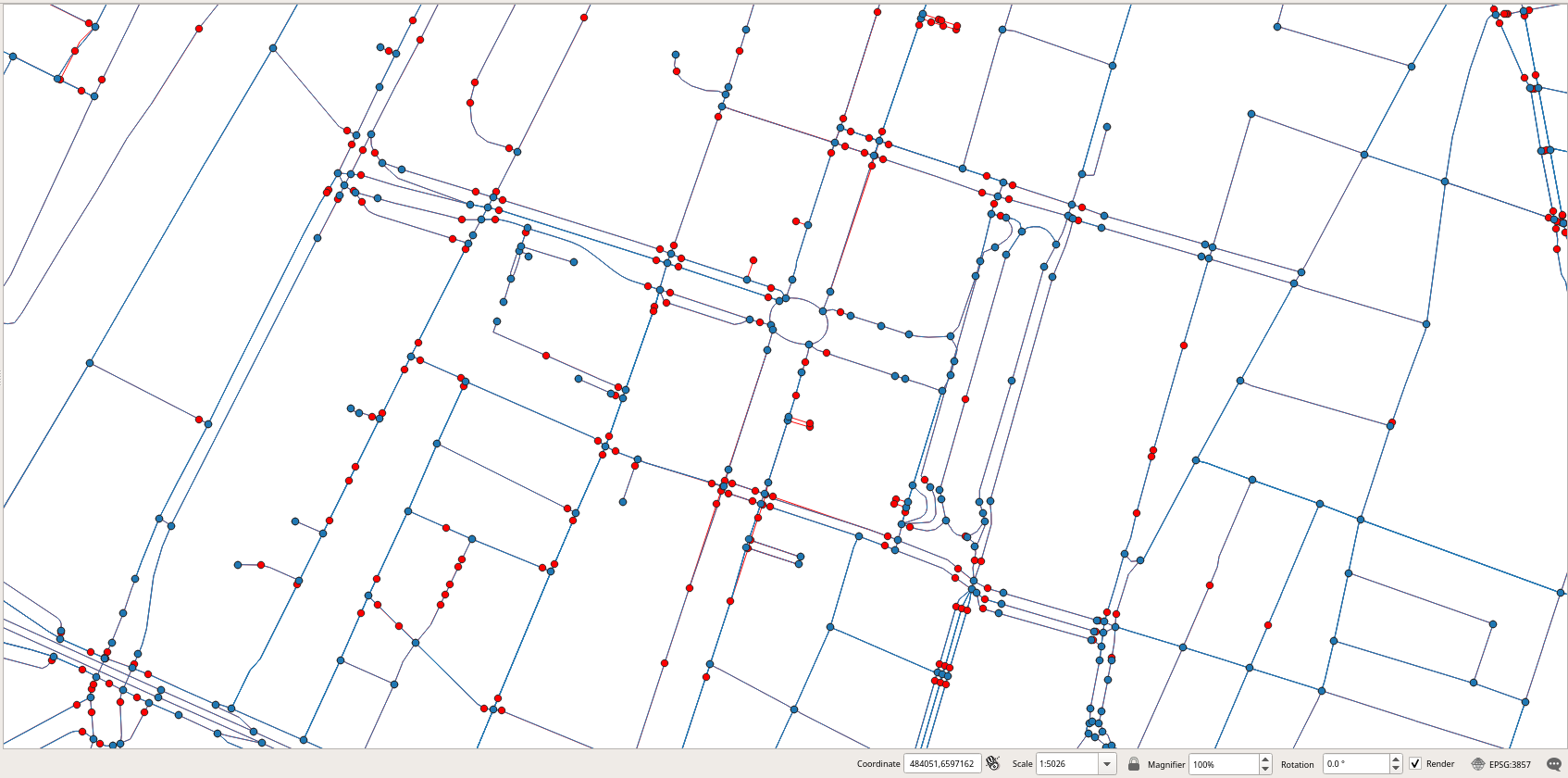
As can be seen, we have reduced the size of the graph. This can also be shown in Figure 2.8, “Comparison of the nodes obtained (in blue) with those obtained by osm2pgrouting (in red).”, where the nodes we have obtained are shown in blue and the ones obtained by osm2pgrouting are shown in red. It can be seen that osm2pgrouting adds many more nodes to the graph, in particular, at the intersection of a road and a pedestrian crossing. Our method only adds nodes when there is an intersection between two roads. We will show in the next section how this network can still be optimized by removing unnecessary nodes and merging the corresponding edges.

Figure 2.8. Comparison of the nodes obtained (in blue) with those obtained by osm2pgrouting (in red).

We show next a possible approach to contract the graph. This approach corresponds to linear contraction provided by pgRouting although we do it differently by taking into account the type, the direction, and the geometry of the roads. For this, we get the initial roads to merge as we did previously but now we put them in a table TempRoads.

DROP TABLE IF EXISTS TempRoads;
CREATE TABLE TempRoads AS
SELECT osm_id, admin_level, bridge, cutting, highway, junction, name, oneway, operator,
  ref, route, surface, toll, tracktype, tunnel, width, way AS Geom
FROM planet_osm_line
WHERE highway IN (SELECT type FROM RoadTypes);
-- SELECT 37045
CREATE INDEX TempRoads_geom_idx ON TempRoads USING GiST(Geom);

Then, we use the following procedure to merge the roads.

CREATE OR REPLACE FUNCTION mergeRoads()
RETURNS void LANGUAGE PLPGSQL AS $$
DECLARE
  i integer = 1;
  cnt integer;
BEGIN
  -- Create tables
  DROP TABLE IF EXISTS MergedRoads;
  CREATE TABLE MergedRoads AS
  SELECT *, '{}'::bigint[] AS Path
  FROM TempRoads;
  CREATE INDEX MergedRoads_geom_idx ON MergedRoads USING GIST(Geom);
  DROP TABLE IF EXISTS Merge;
  CREATE TABLE Merge(osm_id1 bigint, osm_id2 bigint, Geom geometry);
  DROP TABLE IF EXISTS DeletedRoads;
  CREATE TABLE DeletedRoads(osm_id bigint);
  -- Iterate until no geometry can be extended
  LOOP
    RAISE INFO 'Iteration %', i;
    i = i + 1;
    -- Compute the union of two roads
    DELETE FROM Merge;
    INSERT INTO Merge
    SELECT R1.osm_id AS osm_id1, R2.osm_id AS osm_id2,
      ST_LineMerge(ST_Union(R1.Geom, R2.Geom)) AS Geom
    FROM MergedRoads R1, TempRoads R2
    WHERE R1.osm_id <> R2.osm_id AND R1.highway = R2.highway AND
      R1.oneway = R2.oneway AND ST_Intersects(R1.Geom, R2.Geom) AND
      ST_EndPoint(R1.Geom) = ST_StartPoint(R2.Geom) AND NOT EXISTS (
        SELECT * FROM TempRoads R3
        WHERE osm_id NOT IN (SELECT osm_id FROM DeletedRoads) AND
          R3.osm_id <> R1.osm_id AND R3.osm_id <> R2.osm_id AND
          ST_Intersects(R3.Geom, ST_StartPoint(R2.Geom)) ) AND
      geometryType(ST_LineMerge(ST_Union(R1.Geom, R2.Geom))) = 'LINESTRING'
      AND NOT St_Equals(ST_LineMerge(ST_Union(R1.Geom, R2.Geom)), R1.Geom);
    -- Exit if there is no more roads to extend
    SELECT count(*) INTO cnt FROM Merge;
    RAISE INFO 'Extended % roads', cnt;
    EXIT WHEN cnt = 0;
    -- Extend the geometries
    UPDATE MergedRoads R SET
      Geom = M.Geom,
      Path = R.Path || osm_id2
    FROM Merge M
    WHERE R.osm_id = M.osm_id1;
    -- Keep track of redundant roads
    INSERT INTO DeletedRoads
    SELECT osm_id2 FROM Merge
    WHERE osm_id2 NOT IN (SELECT osm_id FROM DeletedRoads);
  END LOOP;
  -- Delete redundant roads
  DELETE FROM MergedRoads R USING DeletedRoads M
  WHERE R.osm_id = M.osm_id;
  -- Drop tables
  DROP TABLE Merge;
  DROP TABLE DeletedRoads;
  RETURN;
END; $$

The procedure starts by creating a table MergedRoads obtained by adding a column Path to the table TempRoads created before. This column keeps track of the identifiers of the roads that are merged with the current one and is initialized to an empty array. It also creates two tables Merge and DeletedRoads that will contain, respectively, the result of merging two roads, and the identifiers of the roads that will be deleted at the end of the process. The procedure then iterates while there is at least one road that can be extended with the geometry of another one to which it connects to. More precisely, a road can be extended with the geometry of another one if they are of the same type and the same direction (as indicated by the attributes highway and one_way), the end point of the road is the start point of the other road, and this common point is not a crossing, that is, there is no other road that starts and this common point. Notice that we only merge roads if their resulting geometry is a linestring and we avoid infinite loops by verifying that the merge of the two roads is different from the original geometry. After that, we update the roads with the new geometries and add the identifier of the road used to extend the geometry into the Path attribute and the DeletedRoads table. After exiting the loop, the procedure finishes by removing unnecessary roads.

The above procedure iterates 20 times for the largest segment that can be assembled, which is located in the ring-road around Brussels between two exits. It takes 15 minutes to execute in my laptop.

INFO:  Iteration 1
INFO:  Extended 3431 roads
INFO:  Iteration 2
INFO:  Extended 1851 roads
INFO:  Iteration 3
INFO:  Extended 882 roads
INFO:  Iteration 4
INFO:  Extended 505 roads
[...]
INFO:  Iteration 17
INFO:  Extended 3 roads
INFO:  Iteration 18
INFO:  Extended 2 roads
INFO:  Iteration 19
INFO:  Extended 1 roads
INFO:  Iteration 20
INFO:  Extended 0 roads

After we apply the above procedure to merge the roads, we are ready to create a new set of roads from which we can construct the graph.

CREATE TABLE Roads AS
SELECT osm_id || Path AS osm_id, admin_level, bridge, cutting, highway, junction, name,
  oneway, operator, ref, route, surface, toll, tracktype, tunnel, width, Geom
FROM MergedRoads;

CREATE INDEX Roads_geom_idx ON Roads USING GiST(Geom);

Notice that now the attribute osm_id is an array of OSM identifiers (which are big integers), whereas in the previous section it was a single big integer.

We then proceed as we did in the section called “Creating the Graph” to compute the set of nodes and the set of edges, which we will store now for comparison purposes into tables Nodes1 and Edges1. We can issue the following queries to compare the two graphs we have obtained and the one obtained by osm2pgrouting .

SELECT count(*) FROM Ways;
-- 83017
SELECT count(*) FROM Edges;
-- 81073
SELECT count(*) FROM Edges1;
-- 77986
SELECT count(*) FROM Ways_vertices_pgr;
-- 66832
SELECT count(*) FROM Nodes;
-- 45494
SELECT count(*) FROM Nodes1;
-- 42156

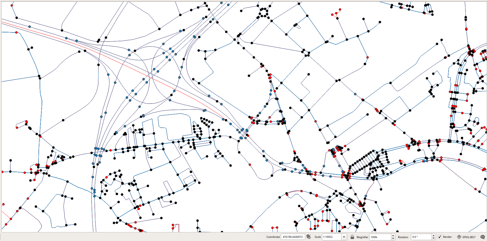
Figure 2.9, “Comparison of the nodes obtained by contracting the graph (in black), before contraction (in blue), and those obtained by osm2pgrouting (in red).” shows the nodes for the three graphs, those obtained after contracting the graph are shown in black, those before contraction are shown in blue, and those obtained by osm2pgrouting are shown in red. The figure shows in particular how several segments of the ring-road around Brussels are merged together since the have the same road type, direction, and maximum speed, The figure also shows in read a road that was removed since it does not belong to the strongly connected components of the graph.

Figure 2.9. Comparison of the nodes obtained by contracting the graph (in black), before contraction (in blue), and those obtained by osm2pgrouting (in red).