Now we are ready to construct ship trajectories out of their individual observations:

CREATE TABLE Ships(MMSI, Trip, SOG, COG) AS 
SELECT MMSI, 
  tgeompointSeq(array_agg(tgeompoint(ST_Transform(Geom, 25832), T) ORDER BY T)), 
  tfloatSeq(array_agg(tfloat(SOG, T) ORDER BY T) FILTER (WHERE SOG IS NOT NULL)), 
  tfloatSeq(array_agg(tfloat(COG, T) ORDER BY T) FILTER (WHERE COG IS NOT NULL)) 
FROM AISInputFiltered 
GROUP BY MMSI;
-- Query returned successfully: 6264 rows affected, 00:52 minutes execution time.

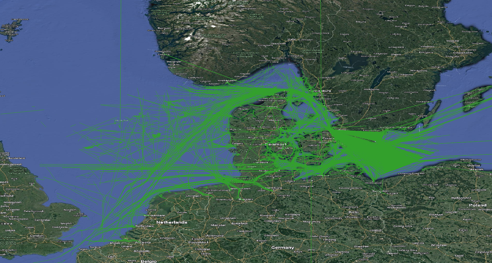
This query constructs, per ship, its spatiotemporal trajectory Trip, and two temporal attributes SOG and COG. Trip is a temporal geometry point, and both SOG and COG are temporal floats. MobilityDB builds on the coordinate transformation feature of PostGIS. Here the SRID 25832 (European Terrestrial Reference System 1989) is used, because it is the one advised by Danish Maritime Authority in the download page of this dataset. Figure 1.2, “Visualizing the ship trajectories” shows the constructed trajectories in QGIS.

ALTER TABLE Ships ADD COLUMN Traj geometry;
UPDATE Ships SET Traj = trajectory(Trip);
-- Query returned successfully: 6264 rows affected, 3.8 secs execution time.

Figure 1.2, “Visualizing the ship trajectories” shows the constructed trajectories in QGIS. Notice that there are still significant errors in the data, in particular the vertical lines. These errors need to be corrected so that the analytical queries in the following sections return more accurate results. We do not cope with this issue here, since the topic of trajectory cleaning is beyond the scope of this introductory workshop.

Figure 1.2. Visualizing the ship trajectories